How to show Charts with Hidden Data Cells in Excel
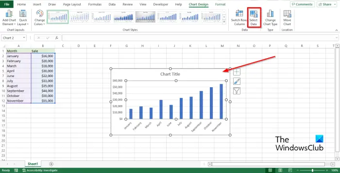
When there is data that is hidden in your table, Excel will not show that information in the chart. Follow the steps below to show charts with hidden data cells in Excel. In this tutorial, you will notice that the data for May is hidden.
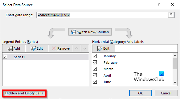
Select the chart, then click the Chart Design tab. Click the Select Data button in the Data group. The Select Data feature changes the data range included in the chart. A Select Data Source dialog box will open.
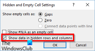
Click the Hidden and empty cells button. A Hidden and empty cells settings dialog box will open.
Click the Show data in hidden rows and columns check box, then click OK for both dialog boxes.
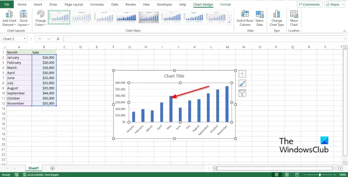
You will notice that the May information that was missing is now shown in the chart. We hope you understand how to show charts with hidden data in Excel.
How do I remove extra data from Excel chart?
Follow the steps below on how to remove extra data from an Excel Chart. READ: How to create a Lollipop Chart in Excel
How do I get a chart to ignore blank cells?
Follow the steps below on how to ignore blank cells in Excel: READ: How to move and resize a Chart in Excel.