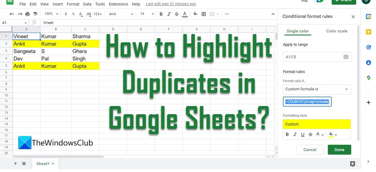
In this article, we are going to show you how to highlight duplicates in Google Sheets in the following ways:
How to Highlight Duplicates in Google Sheets?
We are going to use the COUNTIF function to highlight duplicates in Google Sheets. The COUNTIF function counts across columns, row-by-row. The syntax of the COUNTIF function is: f(x)=COUNTIF(range, criterion) Where range refers to the cell range on which the function needs to be applied and criterion refers to the condition which needs to be met. The COUNTIF function returns TRUE or FALSE based on the match. Now let’s see how the formula works in Google Sheets.
1] Highlight duplicate cells in a single column in Google Sheets
Let’s say we have a spreadsheet with some names written in it. The sheet contains some duplicate name entries which we are going to find and highlight using the COUNTIF function and conditional formatting in Google Sheets. Open the spreadsheet you would like to work on. Click on the Format menu on top of the spreadsheet. Select Conditional formatting.
You’ll see the Conditional format rules panel on the right side of the screen. Click on the icon next to the Apply to range option and use your mouse pointer to select a data range. For the dataset shown in the above image, we have set the range to A1:A10.
Select Custom formula is under the Format rules dropdown and enter the COUNTIF function in the value or formula textbox.
We have used the following formula for the above dataset: f(x)=COUNTIF($A$1:$A$10,$A1)>1 In this formula, the condition has been set as $A1. The $ sign locks a column/row and tells the formula to count cells only from the specified column/ row. So the $ sign here indicates that the condition is based on column A only. This will pick a cell value from column A (A1, A2, and so on), match it with all other cell values in column A and return True if a match is found. By adding >1, we are further highlighting all the instances of duplicates found within column A. By default, the cells will be highlighted in a shade close to light blue. You can select custom colors under the Formatting style option to highlight cells in the color of your choice. We have highlighted duplicates in yellow color in our example.
Click on the Done button to close the Conditional format rules panel.
2] Highlight the entire row if duplicates are in one Google Sheets column
Using the same formula, we can highlight the entire row if duplicates are in one Google Sheets column. The only change here would be the selected range (Apply to range). We have selected A1:C10 here, so conditional formatting will highlight the entire row, instead of highlighting individual cells. Also Read: How to count checkboxes in Google Sheets.
3] Highlight duplicate cells in multiple Google Sheets columns
We can adjust the same formula to highlight duplicate cells in multiple Google Sheets columns. We are making the following 2 changes to the formula: After removing the $ sign, the formula will count cells from all the columns, including columns A, B, C, and so on. For the dataset shown in the above image, the formula will be: f(x)=COUNTIF($A$1:$C$5,A1)>1
4] Highlight actual duplicates, leaving the 1st instance
Again, we can use the same formula to highlight actual duplicates by ignoring the 1st instance. For this, we need to lock the column in the end range, but not the row. In this arrangement, each row will look for duplicates in its above rows only. For the dataset shown in the above example, we have used the following formula: f(x)=COUNTIF($A$1:$A1,$A1)>1
5] Highlight complete row duplicates in Google Sheets
We can use ArrayFormula with COUNTIF to highlight complete row duplicates in Google Sheets. ArrayFormula concatenates the data in multiple columns in a single string before applying the COUNTIF rule. So for the above dataset, the function will be: f(x)=COUNTIF(ArrayFormula($A$1:$A$5&$B$1:$B$5&$C$1:$C$5),$A1&$B1&$C1)>1 This sums up different ways of highlighting duplicate cells in Google Sheets. Hope you find this useful.
How do I find duplicates in Google Sheets?
Google Sheets offers flexible ways to find, review or fix duplicate data. For example, you can highlight a single cell carrying the duplicate value, or the entire row of data if there’s a duplicate in a particular column. Duplicates can be highlighted based on a condition and conditional formatting rules. The condition may be defined using a custom formula, such as COUNTIF. Refer to the above article to learn how to use the COUNTIF function in Google Sheets.
How do I highlight duplicates in columns?
Suppose we have a spreadsheet containing data in the cell range A1:C5. To highlight duplicates in multiple columns in this dataset, we may use the COUNTIF function as, f(x)=COUNTIF($A$1:$C$5,A1)>1. This will pick a cell in a column, compare it with the rest of the cells and return TRUE if a match is found. The comparison will happen for each column in the dataset.
How do I edit a rule in conditional formatting?
Follow the steps to edit a rule in conditional formatting in Google Sheets: To apply another rule on the same range, you may use the ‘Add another rule’ option. To delete a rule, you can click on the trash icon next to the rule. Read Next: How to install Custom Fonts on Google Docs.
