How to hide Formula in Excel
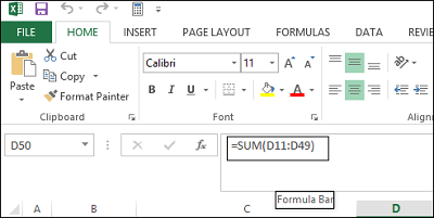
The formulas are displayed in the formula bar as shown in the screenshot below. Alternatively, to display the formula, you can click ‘Show Formulas’ in the Formula Auditing section of the Formulas tab.
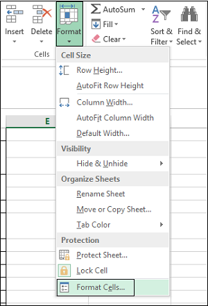
If you don’t want the formulas visible to users viewing your spreadsheet, you can hide them and protect the sheet. To do this, select the cells whose formulas you want to hide. Next, move to ‘Home’ tab. Look for the Cells section to the Right. From this section, choose Format and select Format Cells from the drop-down menu.
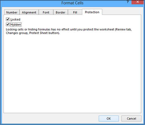
Instantly, the Format Cells dialog box should pop up on your computer screen. When this happens, switch to ‘Protection’ tab. There, select the Hidden check box and Hit ‘OK’.
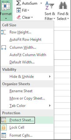
The final step is to protect your Excel Worksheet to finish hiding the formulas. Click Format in the Cells section of the Home tab again. Now, select Protect Sheet from the drop-down menu.
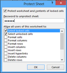
When presented with the dialog box, make sure the contents of locked cells and the Protect worksheet check box is selected. You will be required to enter a password in the Password field.
Enter your password again in the Reenter password to proceed edit box on the Confirm Password dialog box and click OK. At any stage, should you feel to unprotect the sheet and show the formulas again, select Unprotect sheet option and enter the saved password in Unprotect Sheet password box. In the Allow all users of this worksheet to list box, select the check boxes for the tasks you want to allow the users to perform. Click OK. Now see how you van make the best use of Name Box in Excel.
