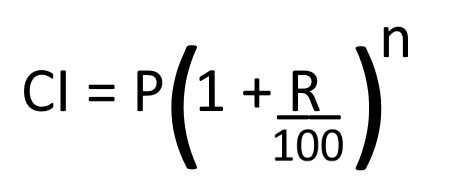
Apart from calculating the compound interest on paper, if you know how to calculate it in Excel, it will be an added advantage to your professionalism. In the above formula, P stands for the principal value, R is the rate of interest, and n is total time. Here, we will learn to calculate compound interest using Excel. But before we begin, let’s have a look at the terms used in compound interest calculations.
Compounded annually or yearly: Here, the rate of interest is applied to the principal value every year.Compounded half-yearly or semi-annually: Here, the principal value is increased after every 6 months, which means two times a year. To calculate compound interest half-yearly, we have to multiply n by 2 and divide the rate by 2.Compounded quarterly: Every year has four quarters. Here, the principal value gets increased after every 3 months, which means 4 times a year. To calculate compound interest quarterly, we have to multiply n by 4 and divide the rate of interest by 4.Compounded monthly: There are 12 months in a year. Therefore, compounded monthly means the interest is applied every month. Hence, we have to multiply the n by 12 and divide the rate of interest by 12.
How to calculate Compound Interest (CI) in Excel
We will discuss here: Let’s see the calculation of compound interest in Excel.
1] Calculating Interest Compounded Annually in Excel
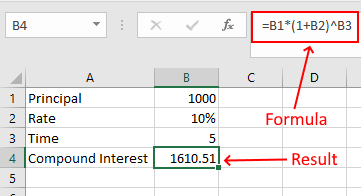
Let’s take a sample data with the following values:
P = 1000R = 10%n = 5 years
Enter the above data in Excel and write the following formula: B1, B2, and B3 are the cell addresses that indicate principal value, rate of interest, and time respectively. Please enter the cell address correctly, otherwise, you will get an error.
2] Calculating Interest Compounded Half-yearly in Excel
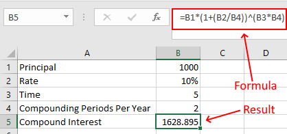
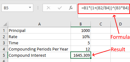
Here, we have to add one more value to our data, compounding periods per year. As explained above, two half years make a complete year. Therefore, there are 2 compounding periods in half-yearly.
Principal = 1000Rate of interest = 10%Time = 5 yearsCompounding periods per year = 2
Enter the above data in Excel and write the following formula: See, we have divided the rate of interest (value in the B2 cell) by 2 (value in the B4 cell) and multiplied the time (value on the B3 cell) by 2 (value in the B4 cell).
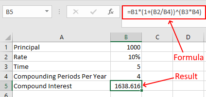
3] Calculating Interest Compounded Quarterly in Excel
Here, the formula remains the same, which we have used in the calculation of CI half-yearly. Now, you just have to change the values in the respective cells. For quarterly CI calculation, change the value of the B4 cell to 4.
4] Calculating Interest Compounded Monthly in Excel
To calculate the interest compounded monthly, change the value of the B4 cell to 12 and use the same formula. That’s it. Let us know if you have any questions regarding the calculation of CI in Excel. Read next: How to Calculate Simple Interest in Excel.